30 January 2017
Background
Motivation
People who poke at DNA or protein sequences as part of their job occaisionally need to find regions that are repetitive or made up of a few nucleic/amino acids. That’s because those regions (1) can have important biological roles such as secondary structure, function, and in the unique case of DNA, expression, and (2) can confuse algorithms such as the BLAST alignment algorithm✪I’m mostly interested in the latter, as I’m trying to speed up BLAST using a Bloom filter. I admit I was dissappointed to find some bright people thought so as well in 2009, but I plan on writing an implementation for the hell of it..
By the end of this article, we’ll write a simple python program to to identify regions that are made of few or repeating amino/nucleic acids (called “low-complexity”), and sequences with less biased distributions (“high-complexity”).
Here is an example of both “low-complexity” (repeating) and “high-complexity” regions from the human major prion protein sequence:
> Low-Complexity
PHGGGWGQPHGGGWGQPHGGGWGQPHGGGWGQ

> High-Complexity
RPIIHFGSDYEDRYYRENMHRYPNQVYYRPMD
Implementation
Well, we’ll base our approach on the one described in (Wooton, 1993), partly because Wooton is fun to say, and partly due to the fact that the author used this approach to write SEG, which is the time-tested de facto tool for identifying low-complexity protein sequences. Our version, however, will use a simplified (although arguably as effective) measure of complexity.
Scanning the Sequence with Sliding Windows
The first thing the SEG algorithm does is scan over a sequence in overlapping (aka “sliding”) windows of size \(L\), whose default value is \(12\). Below is an example sequence and the windows it would yield if \(L=3\):
Sequence: AACTAGCCCGCT
Windows (L=3): ['AAC', 'ACT', 'CTA', 'TAG', 'AGC', 'GCC', 'CCC', 'CCG', 'CGC', 'GCT']
We can implement this easily in python with the following function:
def overlapping_windows(sequence, L):
    """
    Returns overlapping windows of size `L` from sequence `sequence`
    :param sequence: the nucleotide or protein sequence to scan over
    :param L: the length of the windows to yield
    """
    windows = []

    for index, residue in enumerate(sequence):
        if (index + L) < (len(sequence) + 1):
            window = sequence[index:L+index]
            windows.append(window)

    return windows
Repetition Vectors
Now that we have windows, we can translate these sub-sequences into a structure known as a “repetition vector” (or RepVec here)✪Wooton calls these “complexity state vectors”. I also just noticed the word “repetition” is rather compositionally repetitive…. RepVecs are super simple to grok, but I’ll give a bit of a formal definition.
Briefly, if you have a DNA sequence AGCT, it has a RepVec \((1,1,1,1)\), which is the most complex RepVec for this case.
On the other hand, AGCC and GGGG have the complexity sequences \((2,1,1,0)\) and \((4,0,0,0)\) respectively, the
latter being the least complex RepVec for this case.
Slightly more formally, a RepVec has \(N\) entries where \(N\) is the number of residues in a biopolymer (e.g.: \(N=4\) for DNA and \(N=20\) for amino acids). Each element in the sequence represents the frequency of some residue \(n_i\), such that the RepVec contains the frequency of the occurence of every possible residue in the protein or DNA sequence in descending frequency✪It’s important to note that because of this sorting, the position of \(n_i\) in the RepVec does not represent which residue whose frequency it’s reporting, but it’s value relative to the other frequencies.. RepVecs have the following properties, as described by (Wooton, 1993): $$ 0 \geq n_i \geq L, \sum^N_{i=1} n_i = L $$
def sequence_to_repvec(sequence, N):
    """
    Computes the repetition vector (as seen in Wooton, 1993) from a
    given sequence of a biopolymer with `N` possible residues.

    :param sequence: the nucleotide or protein sequence to generate a repetition vector for.
    :param N: the total number of possible residues in the biopolymer `sequence` belongs to.
    """
    encountered_residues = set()
    repvec = []

    for residue in sequence:
        if residue not in encountered_residues:
            residue_count = sequence.count(residue)

            repvec.append(residue_count)

            encountered_residues.add(residue)

        if len(encountered_residues) == N:
            break

    while len(repvec) < N:
        repvec.append(0)

    return sorted(repvec, reverse=True)
Computing Compositional Complexity from a RepVec
Before I get to computing complexity, I’ll first have to first describe something called Shannon Entropy, but briefly: compositional complexity will be measured indirectly using Shannon Entropy. The SEG algorithm adds a couple of more measures and a lot of other logic. If you’re up on your Information Theory, you might want to skip to the code.
While working on cracking Nazi codes at Bell Labs, and well before he was counting cards in Vegas, a flame-throwing trumpet-playing unicycler named Claude E. Shannon described a new kind of Entropy from the thermodynamic one we know.
Shannon’s Entropy describes how unpredictable the contents of a message is.
Examples of low-entropy sequences include outdoor temperature and the English language. The reason being that if you tell me that the mid-day temperature in Montréal today is -10°C, I can tell you that the following day will likely be somewhere between -5°C and -15°C✪via Climate-Data.org.Similarly, certain letters and letter combinations are more common than others in the English language. For example, if the first letter of a word is “q”, the next word is almost guaranteed to be a “u”. Similarly, if I’m to guess the last word of any word, “e” or “s” would be better guesses than “j” or “q”.
Examples of high-entropy sequences include coin flips or dice roles. Knowing that the previous coin-flip was heads or that the previous role of a six-sided die was 4 won’t give you a better idea of what the next coin toss or die-roll will result in.
We can apply this to our DNA since low-compositional-complexity sequences will have low Shannon entropy. That’s because, as we’ve seen in the English language example, sequences made up of few of the total possible or repeating elements (which, if you remember, is our definition of low-compositional-complexity) result in low entropy.
If your familiar with entropy in the thermodynamic sense, you’ll be pretty familiar with the formula for Shannon entropy. The Gibb’s (i.e. thermodynamic) Entropy formula is:
$$ S = -k_b \sum^N_{i=1} p_i \ln(p_i) $$
Where \(S\) is entropy of the macroscopic state, \(k_b\) is the Boltzmann constant, and \(p_i\) is the probability of the \(i^\textrm{th}\) macroscopic state of \(N\) possible macroscopic states.
Shannon’s Entropy, on the other hand, is basically the same, except we nix the Boltzman constant (\(k_b\)) since we’re no longer in the thermodynamic context:
$$ H = -\sum p_i \log_2\left( p_i \right) $$
This time around, \(p_i\) is the probability of the appearance of the \(i^{\text{th}}\) character out of \(N\) possible characters a given message might contain.
We can easily adapt this to our RepVec by letting \(p_i=n_i/L\) and letting the log base equal \(N\) (described earlier in “Computing Compositional Complexity…”).
$$ H = - \sum \dfrac{n_i}{L} \log_N \left(\dfrac{n_i}{L}\right) $$
We can calculate for RepVecs in python as follows:
def sequence_entropy(sequence, N):
    """
    Computes the Shannon Entropy of a given sequence of a
    biopolymer with `N` possible residues. See (Wooton, 1993)
    for more.

    :param sequence: the nucleotide or protein sequence whose Shannon Entropy is to calculated.
    :param N: the total number of possible residues in the biopolymer `sequence` belongs to.
    """
    repvec = sequence_to_repvec(sequence, N)

    L = len(sequence)

    entropy = 0

    for n in repvec:
        # we have to throw away elements whose value is 0 since log(0) is invalid
        if n != 0:
            entropy += -1 * ((n/L)*log((n/L), N))

    return entropy
Using list-comprehensions, we can make this code more concise:
def sequence_entropy(sequence, N):

    repvec = sequence_to_repvec(sequence, N)

    L = len(sequence)

    entropy = sum([-1*(n/L)*log((n/L), N) for n in repvec if n != 0])

    return entropy
Establishing an Entropy Threshold
Now that we’re able to compute the entropy of a sequence window, we need to determine “how low is too low” (i.e.: at what point do we mask a nucleic/amino acid). SEG uses an empirical value, which would be interesting for us to try, but their complexity scoring is a little more complicated than what we’re doing here and as such it isn’t going to help us.
To help us determine the threshold, it’ll help us to first visualise the entropy of a protein sequence. SEG uses the human major prion sequence I used earlier as an example in their docs, so let’s keep using that:
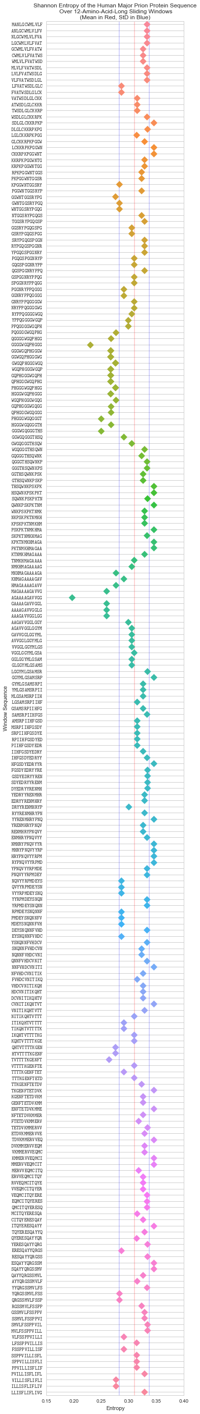
Plotted above are the Shannon entropies of the sliding windows of the human major prion sequence (P04156). The blue lines are the positive and negative standard deviations of the Shannon entropies, and the red line their mean.
There are some notable dips in entropy in the sequence, and the lower standard deviation (the first blue line from left-to-right) looks like as good a place as any to cut them off. It’s not an arbitrary choice, since deviation from the mean is a good way to pick-out outliers in a distribution.
The caveat with this is that very small sequences will give us worse results since the mean and standard deviation are more likely to be further from the population values as the sample size becomes smaller.
Stitching Sequences and Masking Low-Complexity Regions
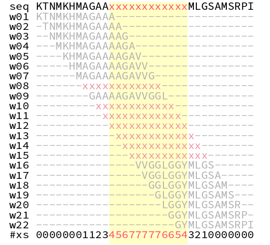
Finally, we put everything together to stitch together the windows, and mask-out regions of low-complexity.
The first step is, for each window, if the window entropy is below the threshold (i.e.: below the first standard deviation), replace all the nucleotides in the window with the mask character (defaults to ‘x’). The second step is to overlay all the windows. Nucleotides that are masked in more than 25% of windows are masked in the final sequence. 25% is a random number, but empirically seems to work. Obviously something you may want to tweak/optimise.
And finally, the python implementation:
def mask_low_complexity(seq, L=12, N=20, maskchar="x"):

    windows = overlapping_windows(seq, L)

    rep_vectors = [(window, compute_rep_vector(window, N)) for window in windows]

    window_complexity_pairs = [(rep_vector[0], complexity(rep_vector[1], N)) for rep_vector in rep_vectors]

    complexities = np.array([complexity(rep_vector[1], N) for rep_vector in rep_vectors])

    avg_complexity = complexities.mean()
    std_complexity = complexities.std()

    k1_cutoff = min([avg_complexity + std_complexity,
                 avg_complexity - std_complexity])

    alignment = [[] for i in range(0, len(seq))]

    for window_offset, window_complexity_pair in enumerate(window_complexity_pairs):

        if window_complexity_pair[1] < k1_cutoff:
            window = "".join([maskchar for i in range(0, L)])

        else:
            window = window_complexity_pair[0]

        for residue_offset, residue in enumerate(window):
            i = window_offset+residue_offset
            alignment[i].append(residue)

    new_seq = []

    for residue_array in alignment:
        if residue_array.count(maskchar) > 3:
            new_seq.append(maskchar)
        else:
            new_seq.append(residue_array[0])

    new_seq = "".join(new_seq)

    return (new_seq, alignment)
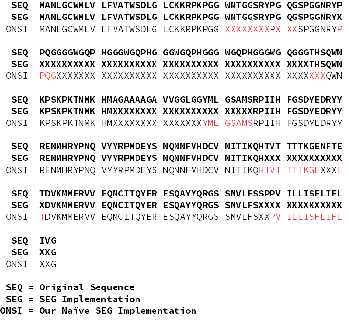
We’ve done it (Woo!), now let’s compare the output of our naïve SEG implementation with that of the genuine article on that Human Prion sequence we’re so fond of:
Discussion
The levenstein distance between SEG and our implementation is 49 (20%), and if you look at the comparison above, the major differences are a couple of nucleotides that flank the regions of low-complexity.
Obviously a limitation of this implementation is that it doesn’t work well on small sequences because of how we use mean entropy as a threshold. The way to work around this is to determine the mean and standard deviation of entropy.
Our choice of window size (\(L=12\)) was based on SEG’s empirical choice. Below you can see the difference between entropy for that Human Prion sequence plotted for window sizes between 4 and 40.
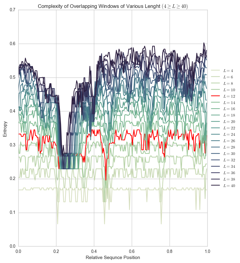
Plots like these can help you pick a window size for a particular sequence, avoiding extremely flat (\(L=4\)) or extremely curvy (\(L=40\)) plots.
What about small sequences?
Because we’re using the lower first standard-deviation as the entropy threshold, we need a significant number of amino/nucleic acids in the sequence. To get around this, we can just pump in as many protein/DNA sequences as we can into the algorithm and calculate the lower first standard-deviation of that… but I’ll call that out-of-scope for this post.